Filters saves the day - gyro drift, accelerometer and derivative noise

The MPU6050 IMU sensor has two distinct sensors - an accelerometer and a gyroscope - both of which works and outputs continuous data streams in its own way. The accelerometer outputs, well acceleration in $m/s^2$ and the gyro outputs angular velocity in $rad/s$.

The problem

Accelerometer data is fast, snappy but noisy. Whereas the gyro is not so snappy, but way less noise tolerance but has something called as Gyro drift. Before that we have to first understand how roll or pitch state is calculated from the gyroscope.

To calculate roll/pitch/yaw - we integrate the gyroscope data with respect to time.

$$\theta = \theta_0 + \int_{0}^{t} \omega \cdot dt$$

Where,

$$\begin{aligned} \theta : \text{current angle} \\ \theta_0: \text{initial angle} \\ \omega: \text{Gyro reading} \end{aligned}$$

So lets say you have pointed the IMU in a way that your heading is along the y-axis then

$$roll = roll_{prev} + \int G_y \cdot (micros() - prevTime)$$

Now, the problem is that just like any sensor, the gyro also has a small bias or noise at absolute zero which accumulates over time during integration, leading to the roll value drifting from the actual reading. 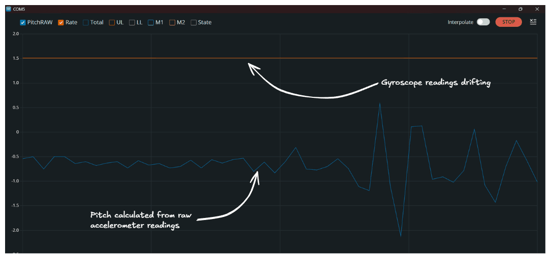The reason why which then we come to something called sensor fusion - combining the sensor data from both the accelerometer and gyroscope streams by adding a weight biases to both.

$$roll = 0.1 \cdot rollA + 0.9 \cdot (roll + G_y \cdot dt)$$

where,

$$\begin{aligned} rollA: \text{angle calculated from accelrometer} \end{aligned}$$

What to do we want ideally - less noise, quick response, zero drift. In the equation above, 10% weightage is given to the accelerometer data and giving the rest to gyro data - and hence the complementary filter. Depending on the project, the weightage can be recalculated to fit objectives.

Derivative noise

After implementing the inner loop for rate control, I noticed that there was huge spikes in the derivative output from the inner loop even due to small noise from the gyro ranging from 0.2-0.5.

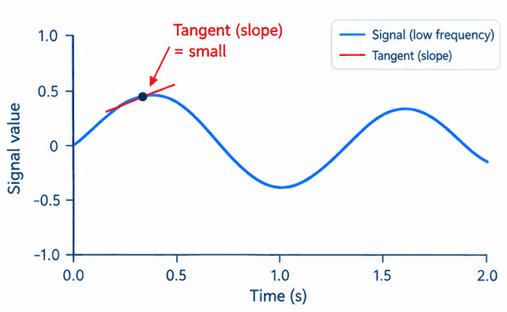
Generated from ChatGPT

Consider a low frequency signal, with a defined amplitude but pretty low frequency and another signal with a higher frequency. Comparing both signals, you will realize that the amplitude may be the same, but the rate of change in initial and final value is higher in the latter case.

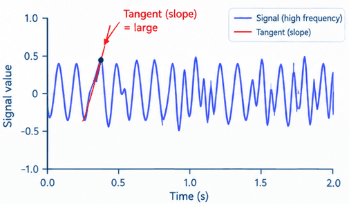
Generated from ChatGPT

The best way to get around this is to implement a software level low pass filter. Consider the equation below for the same

$$D_{filtered}[k] = (1-\alpha)\cdot D_{filtered}[k-1] + \alpha \cdot D_{raw}[k]$$

where,

$$\begin{aligned} & D_{raw} : \text{unfiltered raw derivative noise} \\ & \alpha : \text{cutoff frequency} \end{aligned}$$

Another thing to note is that this derivative noise can be a little more erratic if you increase the bandwidth of the digital low pass filter inside the MPU6050 during setup(), and this is necessary because increasing the bandwidth of the DLPF also improves the response time, which is important for the roll/pitch states. This otherwise can lead to feeding old data during roll & pitch state calculation.